Introduction to Probability
Ad space (future)
Google AdSense block will go here.
Ad space (future)
Google AdSense block will go here.
Probability is a numerical measure of the likelihood that an event will occur. If probabilities are provided, we can determine the likelihood of each event occurring. Probability values are always assigned values between 0 and 1.

When discussing probability, we deal with experiments that have the following characteristics:
The experimental outcomes are well defined, and in many cases are even listed prior to conducting the experiment.
On any single repetition or trial of the experiment, one and only one of the possible experimental outcomes will occur.
The experimental outcome that occurs on any trial is determined solely by chance.
A random experiment is a process that generates well-defined experimental outcomes, and in which on any single repetition, the outcome that occurs is determined completely by chance. For example, the process of tossing a coin or throwing dice is considered a random experiment.
The sample space for a random experiment is the set of all experimental outcomes. An experimental outcome is called a sample point to identify it as an element of the sample space.
For example, tossing a coin has two experimental outcomes or sample points: heads or tails; sample space for rolling dice has six possible sample points: 1,2,3,4,5,6.
Multi-step experiments deal with experiments with multiple steps. For example, throwing two coins. Then possible outcomes are (heads, heads), (heads, tails), (tails, head), (tails, tails).
If an experiment can be described as a sequence of k steps with n1 possible outcomes on the first step, n2 possible outcomes on the second step, and so on, then the total number of experimental outcomes is given by multiplying all n: (n1)(n2)…(nk).
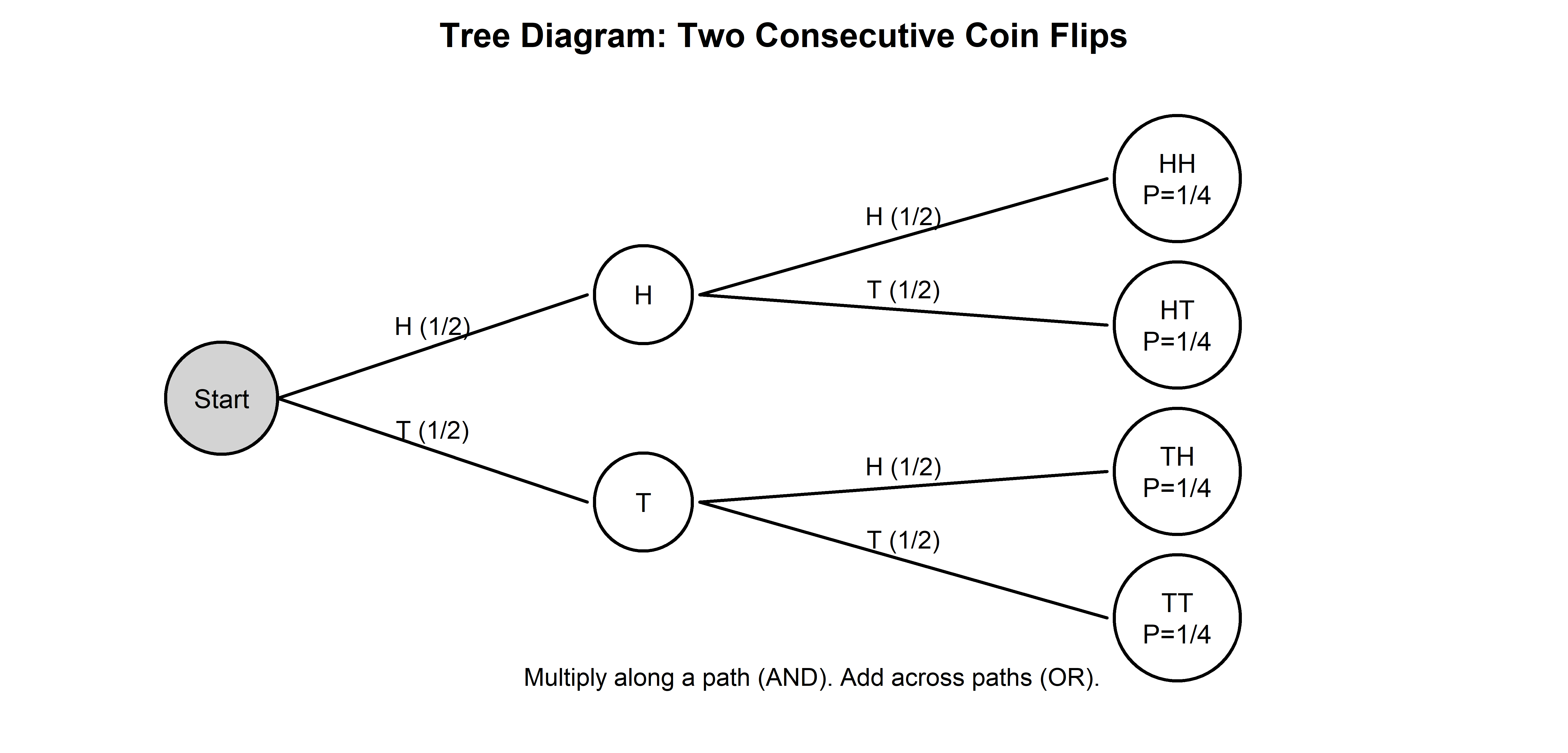
A tree diagram is a graphical representation that helps visualize a multi-step experiment.
A two-consecutive coin flip experiment has two steps: flip a fair coin once, then flip it again. Each flip has two possible outcomes (Heads or Tails), so the tree diagram shows two branches after the first flip, and each of those branches splits again after the second flip. The four possible outcomes (HH, HT, TH, TT) are all equally likely, each with probability 1/4, because we multiply the probabilities along each path ( [1/2] × [1/2] ). To find the probability of an event, we add the probabilities of all paths that correspond to that event (for example, getting exactly one head is HT or TH, so the probability of getting exactly one head is ( [1/4] + [1/4] = 1/2 ).
Counting rules are needed when an experiment has many possible outcomes, making it impractical to list or draw every outcome one by one (as we did with the two-coin example). They give us a fast, systematic way to determine how many outcomes are possible and how many outcomes satisfy an event, which is essential for computing probabilities.
We use counting rules when outcomes are equally likely and the probability of an event can be written as \[ P(event)=\frac{\text{number of outcomes that satisfy an event}}{\text{number of outcomes that are possible}} \]
Counting rules are especially useful when order matters or does not matter.
The counting rule for combinations (used when order is not important) is as described below.
The number of combinations of N objects taken n at a time is as follows:
\[ C^N_n=\frac{N!}{n!(N-n)!} \]
where
\[ N!=N(N-1)(N-2)...(2)(1) \]
\[ n!=n(n-1)(n-2)...(2)(1) \]
\[ 0!=1 \]
In many real-world problems the order of outcomes matters, and different orders lead to different results. Permutations give us a systematic way to count how many ordered arrangements are possible, for situations like passwords, rankings, race finishes, or scheduling where who comes first, second, or third changes the outcome.
The counting rule for permutations (used when order is important) is as described below.
The number of permutations of N objects taken n at a time is as follows:
\[ P^N_n=\frac{N!}{(N-n)!} \]
where
\[ N!=N(N-1)(N-2)...(2)(1) \]
\[ n!=n(n-1)(n-2)...(2)(1) \]
\[ 0!=1 \]
Basic requirements for assigning probabilities:
The probability assigned to each experimental outcome must be between 0 and 1, inclusively.
The sum of all probabilities for all the experimental outcomes must equal 1.
The classical method of assigning probabilities is appropriate when all experimental outcomes are equally likely.
Classical method: 1/n.
The relative frequency method of assigning probabilities is appropriate when data are available to estimate the proportion of the time the experimental outcome will occur if the experiment is repeated a large number of times.
Relative frequency method: divide the number of one experimental outcome by the number of all outcomes.
The subjective method of assigning probabilities is most appropriate when one cannot realistically assume that experimental outcomes are equally likely and when little relevant data are available. It is typically based on experience, intuition, and other often non-quantitative information.
An event is a collection of sample points.
The probability of any event is equal to the sum of the probabilities of the sample points in the event.
Given an event A, the complement of A is defined to be the event consisting of all sample points that are not in A.
\[ P(A)=1-P(A^C) \]
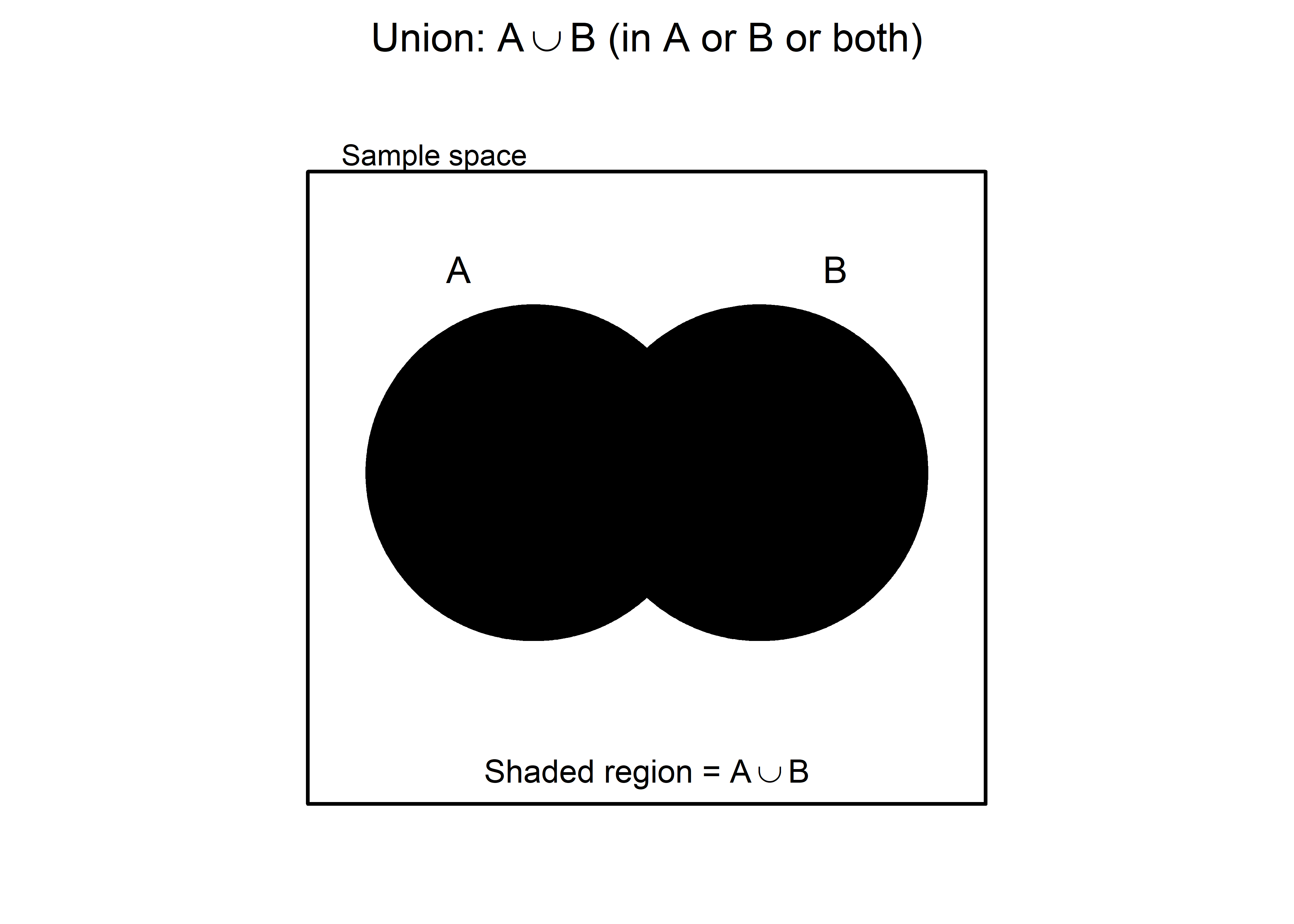
The union of A and B is the event containing all sample points belonging to A or B or both. The union is denoted by \(A\cup B\).
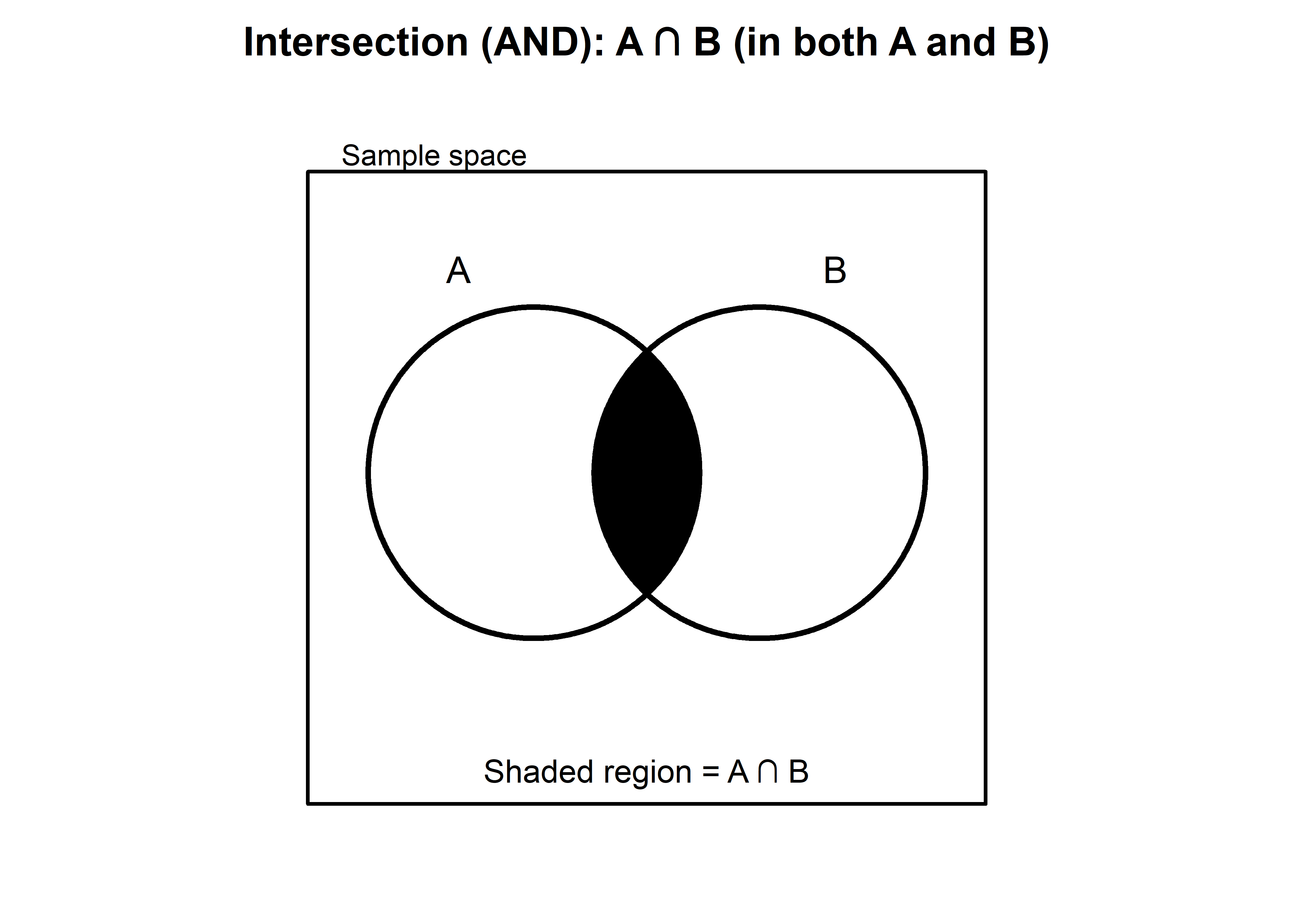
Given two events A and B, the intersection of A and B is the event containing the sample points belonging to both A and B. The intersection is denoted by \(A \cap B\).
The law of addition tells us how to find the probability that at least one of two events occurs (event A or B).
The law of addition: \[ P(A\cup B)=P(A)+P(B)-P(A\cap B) \]
We subtract \(P(A\cap B)\) because outcomes that are in both events would otherwise be counted twice.
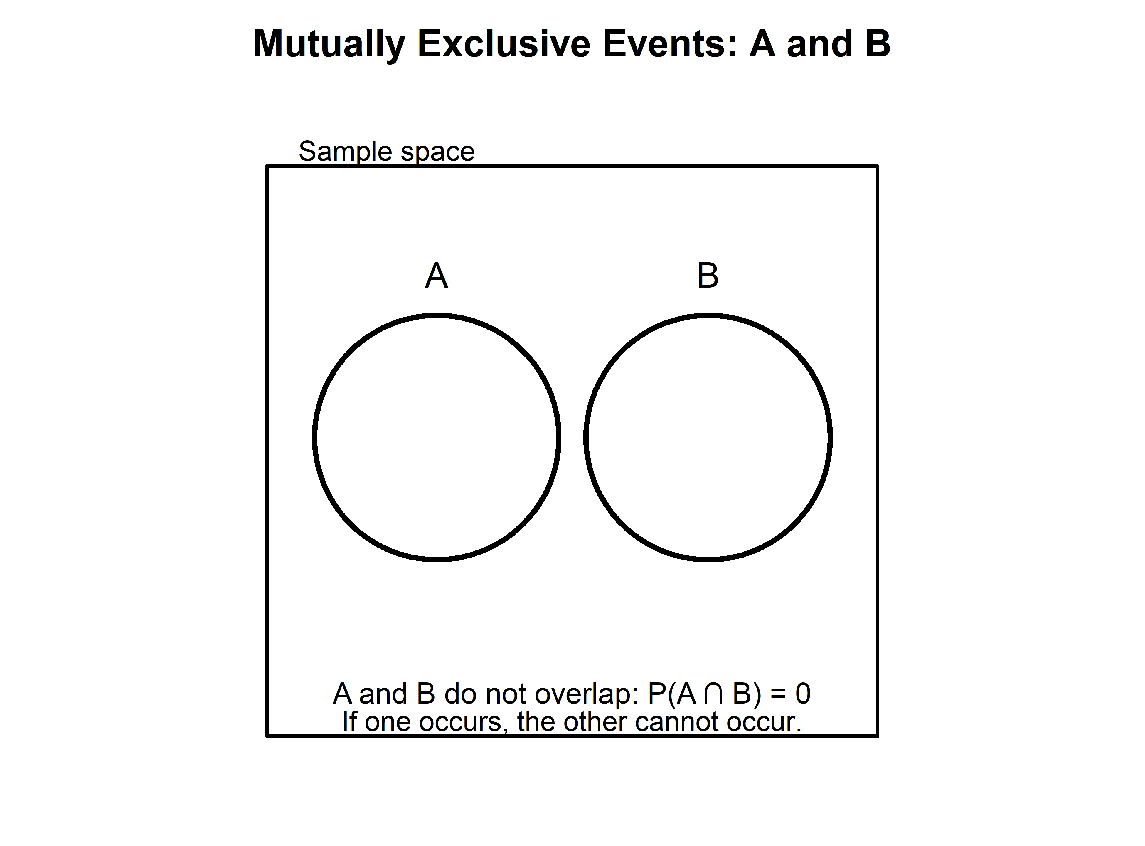
If A and B are mutually exclusive (they cannot occur together), then \(P(A\cap B)=0\), and the rule simplifies to:
\[ P(A\cup B)=P(A)+P(B) \]
The law of addition ensures we count each outcome once and only once when finding the probability of “A or B.”
Often, the probability of an event is influenced by whether a related event already occurred. Say, if we learn that a related event B already occurred, we will want to take advantage of this information by calculating a new probability of event A. This new probability of event A is called a conditional probability and is written \(P(A|B)\) and referred to as the probability of event A given event B (meaning event B occurred).
Conditional Probabilities are defined as follow.
\[ P(A|B)=\frac{P(A\cap B)}{P(B)} \]
\[ P(B|A)=\frac{P(A\cap B)}{P(B)} \]
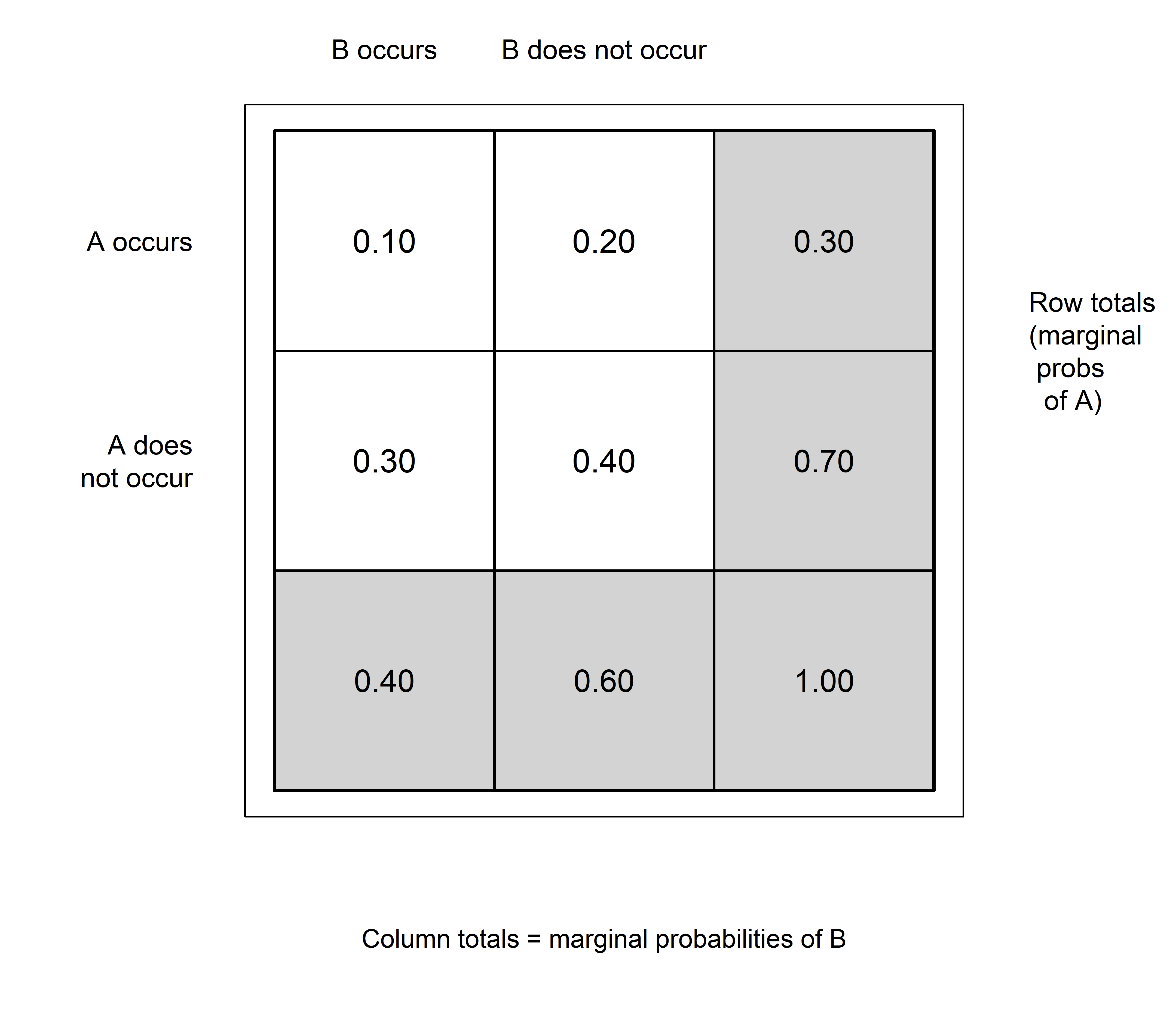
The joint probability table shows the probabilities of an event and the intersection of two events.
Probabilities are called joint probabilities when they give values of probabilities of the intersection of two events (appear inside the joint probability table).
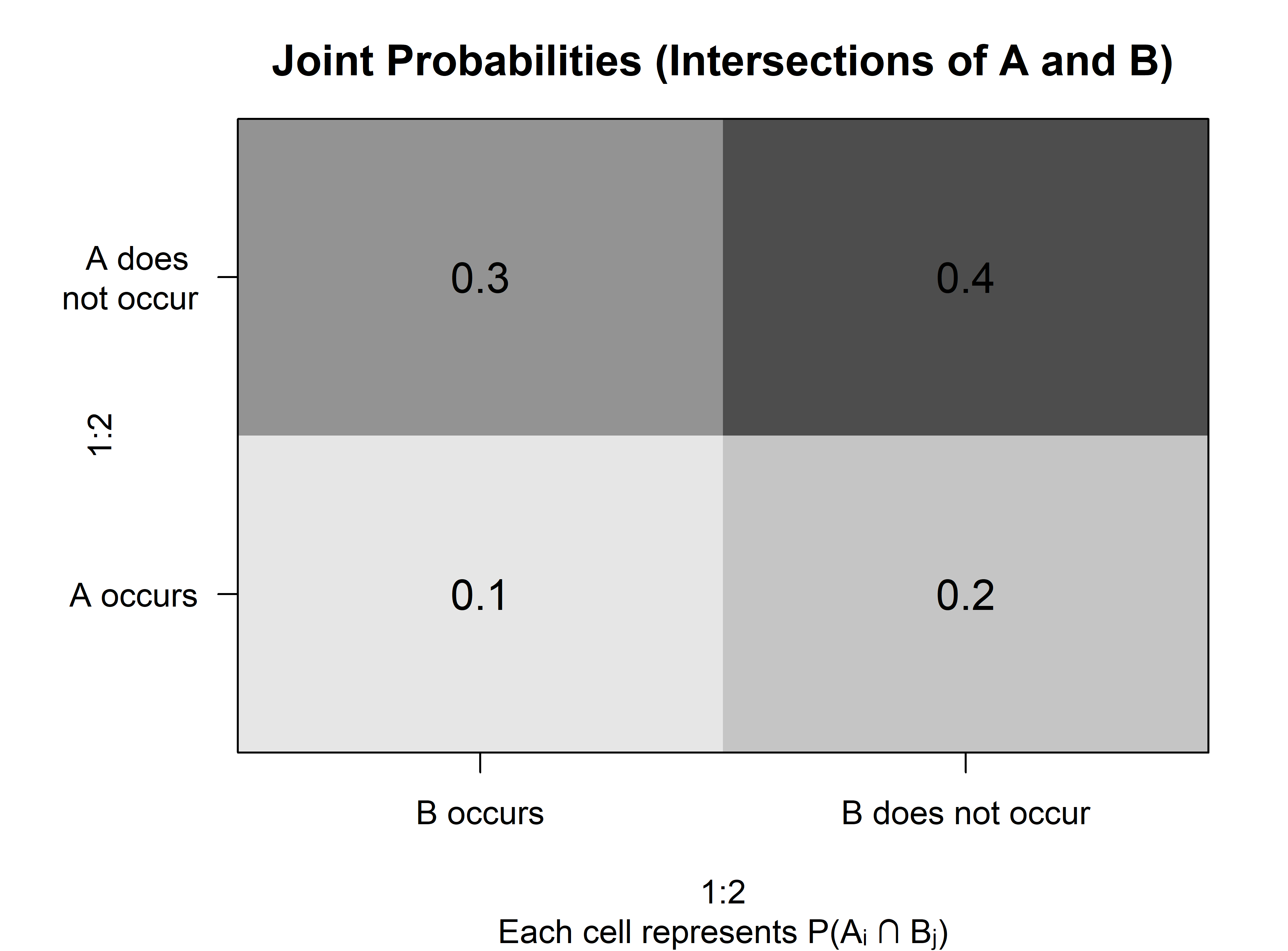
Probabilities are called marginal probabilities when they provide a probability of a specific event (appear in the margins of the joint probability table).
Two events are independent if knowing that one event occurred does not change the probability of the other, meaning.
\[ P(A|B)=P(A) \] \[ P(A\cap B)=P(A)P(B) \]
If this condition does not hold, then events A and B are dependent, because information about one event changes the likelihood of the other.
Independent events and mutually exclusive events describe completely different ideas and are often confused.
Independent events mean that knowing one event occurred does not change the probability of the other. The events can overlap, and in fact, if both events have positive probability, independence requires that they do overlap.
\[ P(A\cap B)=P(A)P(B) \]
Mutually exclusive events mean the events cannot occur together at all, so their overlap is empty. If one mutually exclusive event is known to occur, the probability of other event is reduced to zero. They are therefore dependent.
\[ P(A\cap B)=0 \]
Most real-world events are not independent. For example, the probability of getting hired given an interview is different from the probability of getting hired in general. The general multiplication law lets us correctly compute joint probabilities when one event affects another, preventing serious mistakes in risk assessment, decision-making, and data analysis.
The multiplication law tells us how to find the probability that two events both occur (an AND event). It accounts for the fact that once event A happens, the probability of B may change.
\[ P(A\cap B)=P(A)P(B|A) \]
When events A and B are independent, knowing that one occurred does not change the probability of the other. This simplified rule makes probability calculations much easier but it only works when independence is justified.
\[ P(A\cap B)=P(A)P(B) \]
Revising probabilities when new information is obtained is an important phase of probability analysis. Typically, we begin the analysis with initial or prior probability estimates for specific events of interest. Then, we obtain additional information about the events. Given this new information, we update the prior probability values by calculating revised probabilities which we call posterior probabilities. Bayes’ Theorem provides a means for making these probability calculations.
Consider the following example: there are two suppliers A1 and A2. The probability that a part is good from a supplier is denoted G, bad - B.
Say, that P(A1)=0.65, P(A2)=0.35 (most parts come from supplier A).
Say, that P(G|A1)=0.98, P(B|A1)=0.02 (2% of parts from supplier A are bad).
Say, that P(G|A2)=0.95, P(B|A2)=0.05 (5% of parts from supplier A are bad)
Given that a part is bad, what is the probability that it came from supplier A? To answer this question, we can use Bayes’ Theorem for the two-event case.
Bayes’ Theorem is applicable when the events for which we want to compute posterior probabilities are mutually exclusive and their union is the entire sample.
For the case of N mutually exclusive events, Bayes’ Theorem is as follows:
\[ P(A_1|B)=\frac{P\left(A_1\right)P\left(B|A_1\right)}{P\left(A_1\right)P\left(B|A_1\right)+P\left(A_2\right)P\left(B|A_2\right)} \]
\[ P(A_2|B)=\frac{P\left(A_2\right)P\left(B|A_2\right)}{P\left(A_1\right)P\left(B|A_1\right)+P\left(A_2\right)P\left(B|A_2\right)} \]
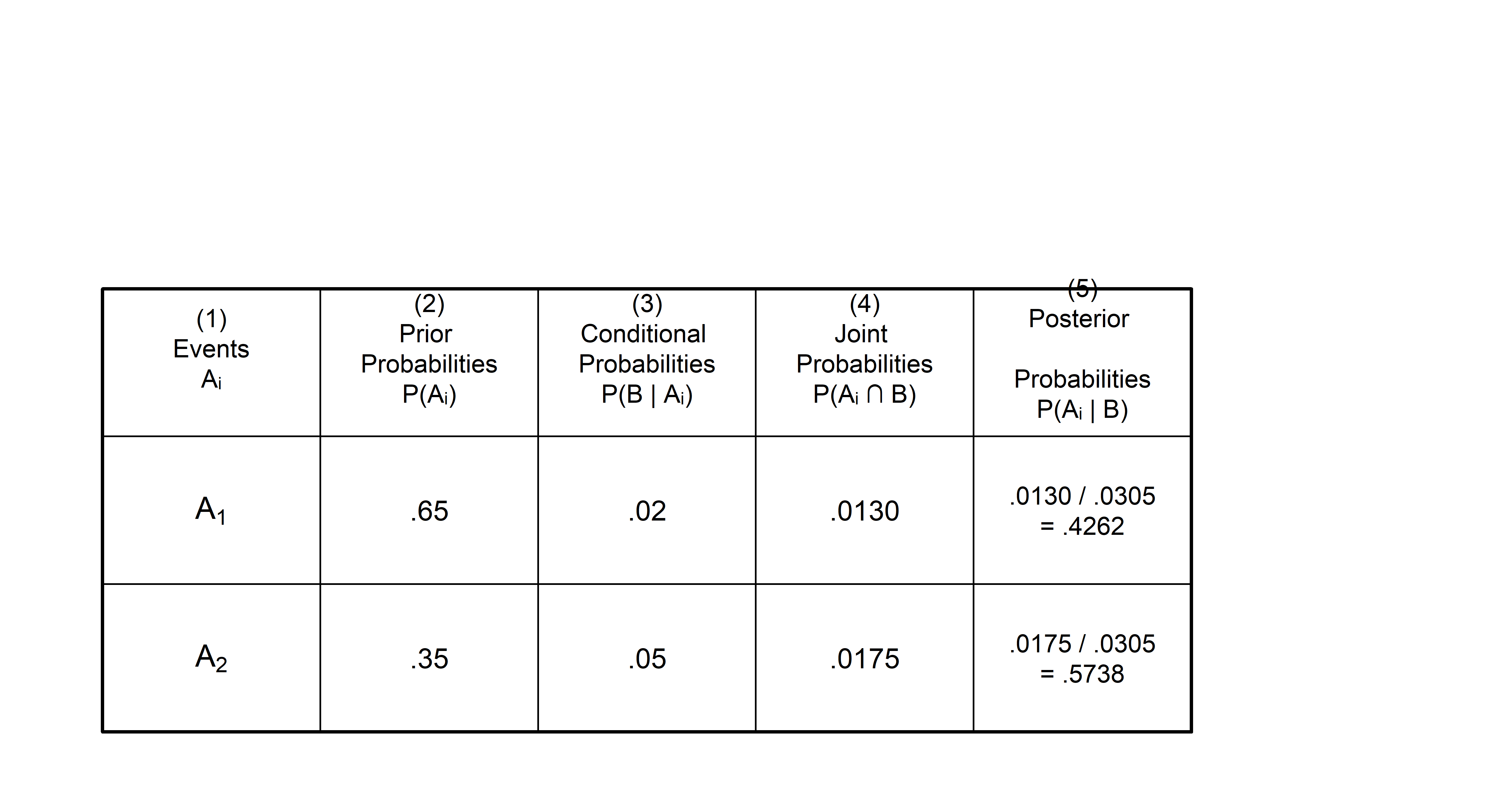
There is also a tabular approach to Bayes’ Theorem calculations.
- Prepare the three columns: Events, Prior Probabilities, Conditional Probabilities
- In column 4, compute the joint probabilities for each event.
- Sum the joint probabilities below the table.
- Compute Posterior Probabilities by dividing each Joint Probability by the Sum of Joint Probabilities.
Practice Problems